l0-Norm, l1-Norm, l2-Norm, … , l-infinity Norm

I’m working on things related to norm a lot lately and it is time to talk about it. In this post we are going to discuss about a whole family of norm.

What is a norm?

Mathematically a norm is a total size or length of all vectors in a vector space  or matrices. For simplicity, we can say that the higher the norm is, the bigger the (value in) matrix or vector is. Norm may come in many forms and many names, including these popular name: Euclidean distance, Mean-squared Error, etc.

Most of the time you will see the norm appears in a equation like this:

where can be a vector or a matrix.

For example, a Euclidean norm of a vector is which is the size of vector

The above example shows how to compute a Euclidean norm, or formally called an -norm. There are many other types of norm that beyond our explanation here, actually for every single real number, there is a norm correspond to it (Notice the emphasised word real number, that means it not limited to only integer.)

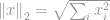
Formally the -norm of is defined as:

 where

That’s it! A p-th-root of a summation of all elements to the p-th power is what we call a norm.

The interesting point is even though every -norm is all look  very similar to each other, their mathematical properties are very different and thus their application are dramatically different too. Hereby we are going to look into some of these norms in details.

l0-norm 

The first norm we are going to discuss is a -norm. By definition, -norm of is

Strictly speaking, -norm is not actually a norm. It is a cardinality function which has its definition in the form of -norm, though many people call it a norm. It is a bit tricky to work with because there is a presence of zeroth-power and zeroth-root in it. Obviously any will become one, but the problems of the definition of zeroth-power and especially zeroth-root is messing things around here. So in reality, most mathematicians and engineers use this definition of -norm instead:

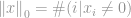
that is a total number of non-zero elements in a vector.

Because it is a number of non-zero element, there is so many applications that use -norm. Lately it is even more in focus because of the rise of the Compressive Sensing scheme, which is try to find the sparsest solution of the under-determined linear system. The sparsest solution means the solution which has fewest non-zero entries, i.e. the lowest -norm. This problem is usually regarding as a optimisation problem of -norm or -optimisation.

l0-optimisation

Many application, including Compressive Sensing, try to minimise the -norm of a vector corresponding to some constraints, hence called “-minimisation”. A standard minimisation problem is formulated as:

subject to

However, doing so is not an easy task. Because the lack of -norm’s mathematical representation, -minimisation is regarded by computer scientist as an NP-hard problem, simply says that it’s too complex and almost impossible to solve.

In many case, -minimisation problem is relaxed to be higher-order norm problem such as -minimisation and -minimisation.

l1-norm

Following the definition of norm, -norm of is defined as

This norm is quite common among the norm family. It has many name and many forms among various fields, namely Manhattan norm is it’s nickname. If the -norm is computed for a difference between two vectors or matrices, that is

it is called Sum of Absolute Difference (SAD) among computer vision scientists.

In more general case of signal difference measurement, it may be scaled to a unit vector by:

where is a size of .

which is known as Mean-Absolute Error (MAE).

l2-norm

The most popular of all norm is the -norm. It is used in almost every field of engineering and science as a whole. Following the basic definition, -norm is defined as

-norm is well known as a Euclidean norm, which is used as a standard quantity for measuring a vector difference. As in -norm, if the Euclidean norm is computed for a vector difference, it is known as a Euclidean distance:

or in its squared form, known as a Sum of Squared Difference (SSD) among Computer Vision scientists:

It’s most well known application in the signal processing field is the Mean-Squared Error (MSE) measurement, which is used to compute a similarity, a quality, or a  correlation between two signals. MSE is

As previously discussed in -optimisation section, because of many issues from both a computational view and a mathematical view, many -optimisation problems relax themselves to become – and -optimisation instead. Because of this, we will now discuss about the optimisation of .

l2-optimisation

As in -optimisation case, the problem of minimising -norm is formulated by

subject to

Assume that the constraint matrix has full rank, this problem is now a underdertermined system which has infinite solutions. The goal in this case is to draw out the best solution, i.e. has lowest -norm, from these infinitely many solutions. This could be a very tedious work if it was to be computed directly. Luckily it is a mathematical trick that can help us a lot in this work.

By using a trick of Lagrange multipliers, we can then define a Lagrangian

where is the introduced Lagrange multipliers. Take derivative of this equation equal to zero to find a optimal solution and get

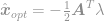
plug this solution into the constraint to get

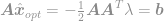
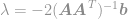
and finally

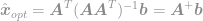
By using this equation, we can now instantly compute an optimal solution of the -optimisation problem. This equation is well known as the Moore-Penrose Pseudoinverse and the problem itself is usually known as Least Square problem, Least Square regression, or Least Square optimisation.

However, even though the solution of Least Square method is easy to compute, it’s not necessary be the best solution. Because of the smooth nature of -norm itself,  it is hard to find a single, best solution for the problem.

In contrary, the -optimisation can provide much better result than this solution.

l1-optimisation

As usual, the -minimisation problem is formulated as

subject to

Because the nature of -norm is not smooth as in the -norm case, the solution of this problem is much better and more unique than the -optimisation.

However, even though the problem of -minimisation has almost the same form as the -minimisation, it’s much harder to solve. Because this problem doesn’t have a smooth function, the trick we used to solve -problem is no longer valid.  The only way left to find its solution is to search for it directly. Searching for the solution means that we have to compute every single possible solution to find the best one from the pool of “infinitely many” possible solutions.

Since there is no easy way to find the solution for this problem mathematically, the usefulness of -optimisation is very limited for decades. Until recently, the advancement of computer with high computational power allows us to “sweep” through all the solutions. By using many helpful algorithms, namely the Convex Optimisation algorithm such as linear programming, or non-linear programming, etc. it’s now possible to find the best solution to this  question. Many applications that rely on -optimisation, including the Compressive Sensing, are now possible.

There are many toolboxes  for -optimisation available nowadays.  These toolboxes usually use different approaches and/or algorithms to solve the same question. The example of these toolboxes are l1-magic, SparseLab, ISAL1,

Now that we have discussed many members of norm family, starting from -norm, -norm, and -norm. It’s time to move on to the next one. As we discussed in the very beginning that there can be any l-whatever norm following the same basic definition of norm, it’s going to take a lot of time to talk about all of them. Fortunately, apart from -, – , and -norm, the rest of them usually uncommon and therefore don’t have so many interesting things to look at. So we’re going to look at the extreme case of norm which is a -norm (l-infinity norm).

l-infinity norm

As always, the definition for -norm is

Now this definition looks tricky again, but actually it is quite strait forward. Consider the vector , let’s say if is the highest entry in the vector  , by the property of the infinity itself, we can say that

 then

then

Now we can simply say that the -norm is

that is the maximum entries’ magnitude of that vector. That surely demystified the meaning of -norm

Now we have discussed the whole family of norm from to , I hope that this discussion would help understanding the meaning of norm, its mathematical properties, and its real-world implication.

Reference and further reading:

Mathematical Norm – wikipedia 

Mathematical Norm – MathWorld

Michael Elad – “Sparse and Redundant Representations : From Theory to Applications in Signal and Image Processing” , Springer, 2010.

 Linear Programming – MathWorld

Compressive Sensing – Rice University

 Edit (15/02/15) : Corrected inaccuracies of the content.